An Introduction to Online Analytical Processing (OLAP)

Online analytical processing (OLAP) software executes detailed analysis on massive volumes of business data, drawn from sources such as data lakes or deep storage. 

End users, such as analysts, executives, and engineers, use OLAP platforms to dissect data around operational performance and profitability, access critical business insights, and steer business or product strategy.

The basics of OLAP

Online analytical processing arose to address a very important need. In order to improve and drive change, organizations need to make sense of their data—through analytics, aggregation, and other operations. 

However, any OLAP software has to overcome several important challenges.

Dispersed data. Due to the diversity of data sources and storage, OLAP systems have to gather and analyze data from various locations. This requires compatibility with a wide range of products, such as data lakes, connectors, streaming data technologies, and more.

Data input via ETL, streaming, and more. When data lives on decentralized storage, an OLAP solution needs to extract data, transform it into a compatible format or structure, and load it, a process known as ETL (more on this later). While this process is still being used, many OLAP systems can also use streaming for data intake, ingesting real-time data events via Amazon Kinesis or Apache Kafka.

Scale. By nature, OLAP architectures are designed to handle large amounts of data. For example, a quarterly report for a multinational corporation will likely involve sifting through terabytes of data. As a result, some OLAP products will include features such as ROLLUP to help compress vast volumes of data into something more manageable.

Resource-intensive operations. Many common OLAP operations, such as drilling down, slicing and dicing, or pivoting, require a lot of computing power. For this reason, OLAP tools have to use parallel processing to accommodate a large number of concurrent users and simultaneous, complex queries.

Speed. Traditionally, OLAP use cases were not time sensitive—quarterly reports, for instance, generally don’t require rapid turnaround times. However, in today’s fast-paced world, those organizations which can rapidly analyze and act on data have an edge over slower competitors, whether it’s a game studio fixing a faulty feature or a digital agency shifting their ad targeting. However, because real-time analytics is still an emerging market, few OLAP solutions are optimized for its demands.

The difference between OLAP and OLTP

For the most part, databases can be divided into two categories: Online Analytical Processing, or OLAP, and Online Transactional Processing, or OLTP. Traditionally, the boundary between the two is clear: whereas OLAP software executes in-depth data analysis to provide business intelligence, OLTP systems handle the day-to-day operations of an organization. Due to their different roles, OLAP databases often work with historical data, while OLTP databases are optimized for real-time data (though this distinction is beginning to blur).

As an analogy, an OLAP system is akin to fitness monitoring for companies. A user can check the health of their organization, see where they excel or fail, devise plans to improve performance, and assess the success of their plans. An OLTP database is the tool that actually implements these strategies, pulling data for transactions, storing records, and verifying interactions between the company and its customers.

This means that OLTP databases can read, write, and delete data rapidly, crucial for meeting real-time demands. In addition, OLTP databases are Atomic, Consistent, Isolated, and Durable, or ACID compliant: basically, transactions are indivisible, discrete operations that do not negatively impact query concurrency or data consistency, and are protected against data loss. This is extremely important for OLTP databases, because many transactions, such as credit card purchases or stock trading, are high volume, fast-paced, and high stakes.

Transactional databases also function differently than analytical ones. Because their data is needed immediately, transactional databases are optimized for lots of rapid, shallow operations. Think of an online retailer retrieving a shipping address for a purchase, or an airline’s automated booking system confirming that connecting times are long enough to permit transfers. In both situations, quick data access is necessary to complete the operation and earn revenue.

Issues arise when OLTP databases are used to perform OLAP duties, or vice versa. In the former case, OLTP software simply doesn’t have the processing power, architecture, or data structures to efficiently execute complex operations like slicing or drilling down, at least not quickly—and not on vast volumes of data. Similarly, OLAP databases cannot carry out lots of fast, small operations involving many parallel users and queries.

Today, the divide between OLTP and OLAP databases remains. However, the rise of real-time analytics, which requires both the ability to accommodate large numbers of concurrent users as well swiftly return results for increasingly complicated queries, is upending this long-running paradigm.

How OLAP databases work

At the most basic level, OLAP systems absorb data from across an environment, transform it into the same format or data type for easier access, and organize this data to ensure fast queries. 

After a data event is generated, it can be stored in a variety of places, including transactional databases like MongoDB or PostgreSQL, or unstructured storage (also known as data lakes) like Amazon S3 or Hadoop. 

For example, a retail point of sale (POS) tablet might generate an event such as a sale, which would live in a transactional database for quick retrieval. After a set period of time, this event would then be automatically moved to a data lake for cold storage, freeing up space in the transactional database for more recent events.

From there, an OLAP product can use any number of ways to ingest data. Some OLAP solutions optimized for rapid, real-time analytics can stream data into their system, either directly from the source (such as a sensor) or via a stream processor (such as Apache Flink), which converts raw event streams into a more digestible configuration.

Alternatively, an OLAP system can ETL the data from a data lake or transactional database. After extracting the data using a connector or other intermediary, the OLAP database would transform it, or prepare the data for analysis by stripping out duplicate readings, filling in missing values, translating it into a different format, and structuring it in columns or tables.

In addition, some OLAP databases ELT their data, extracting and loading it into memory before any transformations. While ETL is often used for large quantities of data, ELT is preferred for smaller data pipelines or environments. 

After data has been imported and added to an OLAP product, it is now ready to be analyzed. One way to do so is the OLAP cube, which despite its name, isn’t necessarily a cube—or even a 3D object. Instead, an OLAP cube is a framework for collecting data across different dimensions and aggregating it for exploration and analysis. 

By including all the relevant data in a single structure, an OLAP system can ensure ease of access, and fast queries, as well as facilitating operations like slice-and-dice, filtering, and more. As a result, OLAP cubes can be more intuitive to use, especially for less-technical employees, who don’t have to write lines of code, SQL statements, or JOIN data tables. The downside is that new reports may require a new cube, as adding too many dimensions to a single cube may risk confusion.

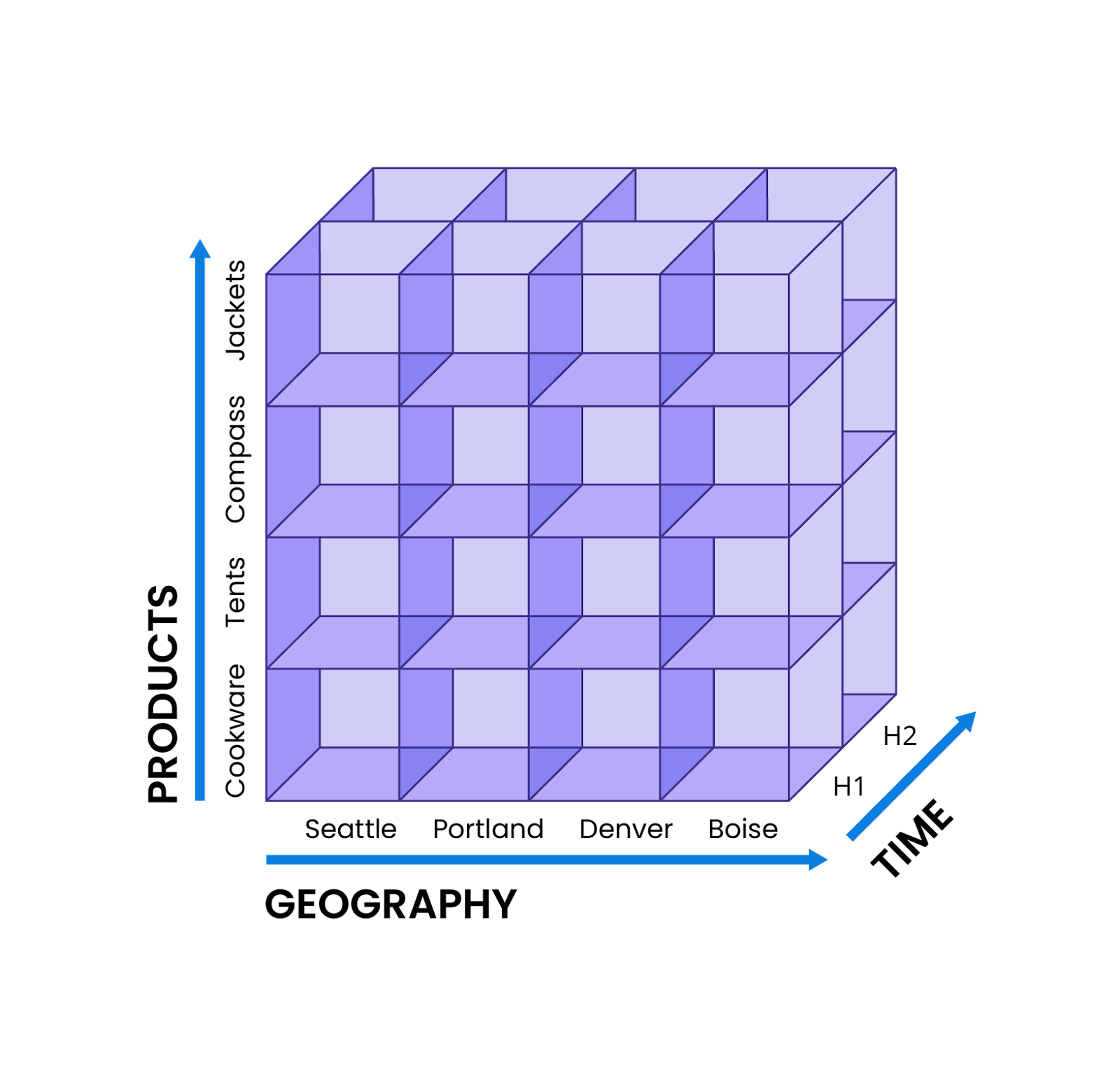
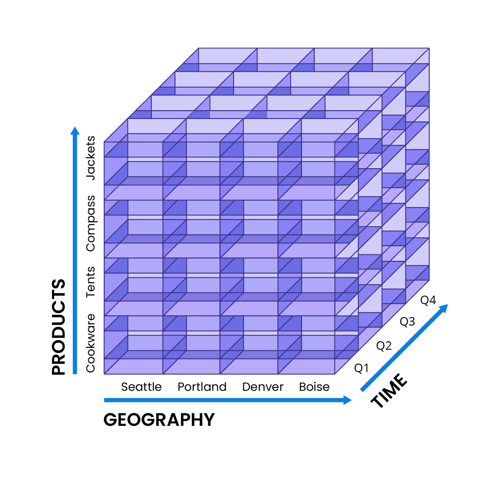
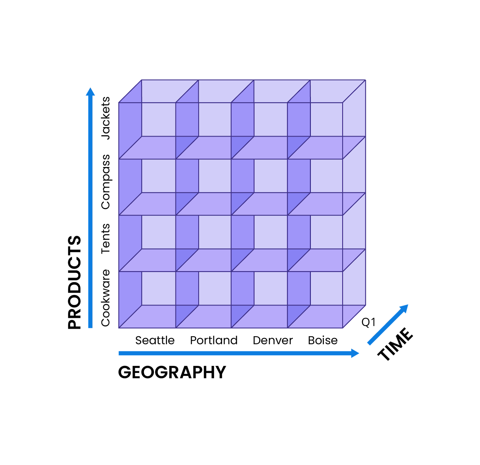
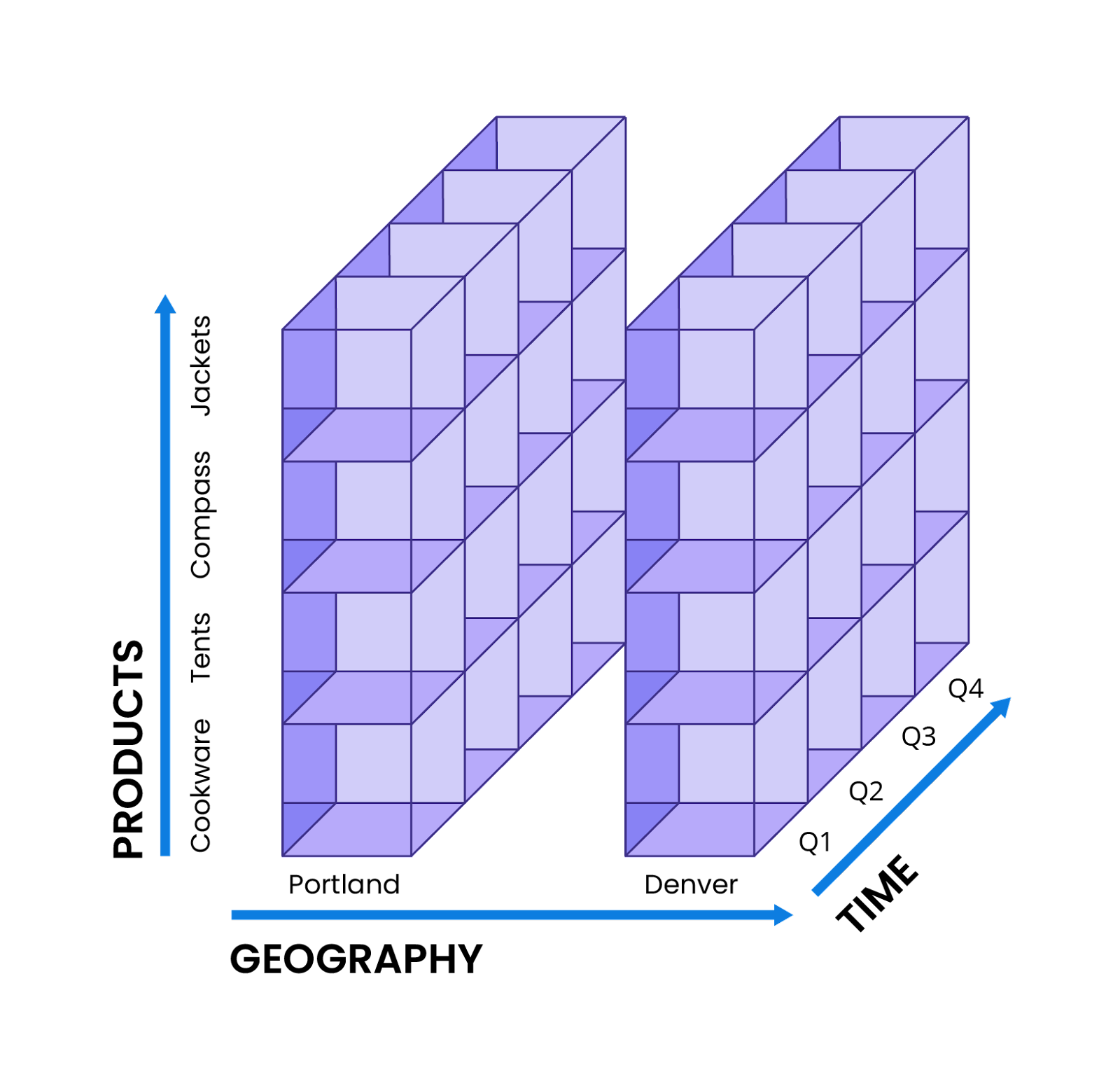
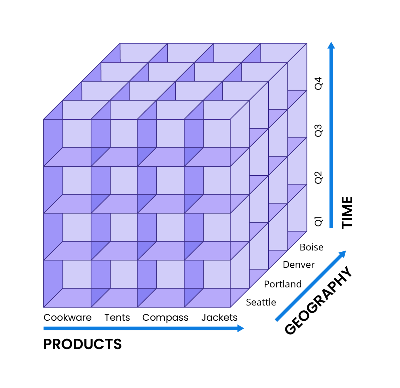
Let’s take the example of an analyst for an outdoor retailer, who’s compiling a yearly sales report. To assemble their cube, this analyst might start by determining the dimensions required, such as the highest selling product categories across their entire business (cookware, tents, compasses, and jackets), the territories in which they sold most successfully, and sales figures by quarters. 

Each dimension would become a separate axis, so that the final cube would be configured in a manner similar to this illustration. 

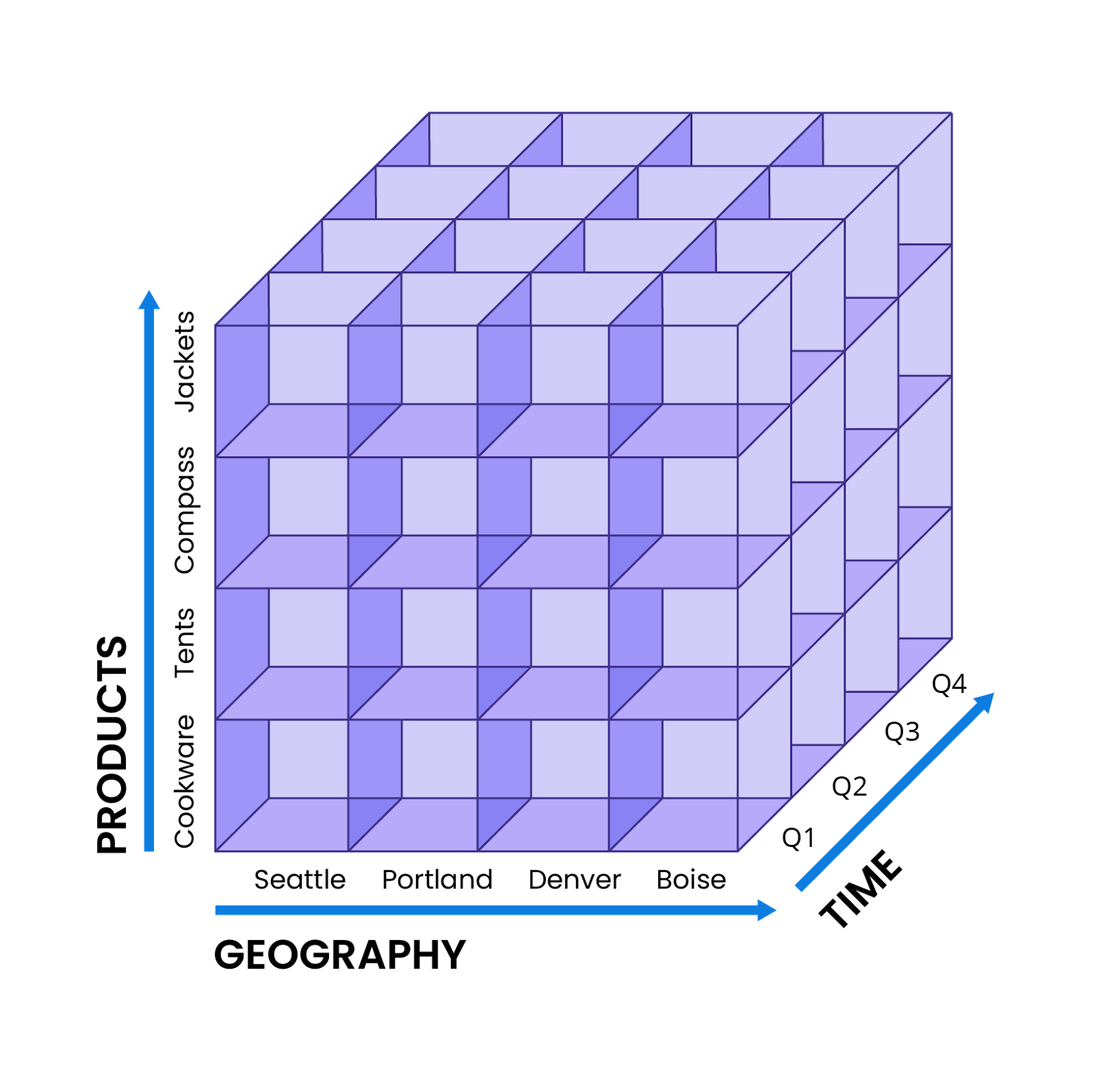
As mentioned above, cubes may have more or less than three axes. If the analyst in this example needs to look at more data, they can do so—adding in dimensions like year-over-year change, buyer demographics such as household income, or even disaggregating each product category into multiple brands.

After data is inputted into a cube, this analyst can run the five core operations featured in all OLAP software:

1. Rollup. By reducing the number of rows or dimensions, rollup compresses and summarizes data, thus saving storage space and reducing costs. Rollup is ideal for situations where high-cardinality values are either scarce or not necessary, or where data granularity can be lengthened (such as setting intervals to one minute instead of one hour). Otherwise, there are a number of ways to compact data without losing detail, such as using sketches to approximate high-cardinality data, rather than using the exact value. To return to our sample e-commerce store, an analyst could rollup sales figures from cities to countries, or from quarters to halves.

2. Drill down. In contrast to rollup, drill down creates more detail and granularity from data. In the previous e-commerce example, the analyst could drill down into their quarterly sales figures to uncover sales revenues by week or month, regional sales figures by city, or best-selling products by brand.

3. Slice. As the name implies, slicing essentially dissects the OLAP cube along a single dimension to provide more specifics. For instance, the e-commerce analyst could slice the OLAP cube to discover the yearly revenue for an individual store in Portland, Oregon. 

4. Dice. Unlike slicing, dicing separates two or more OLAP cube dimensions for in-depth comparisons. As an example, the analyst could compare the yearly revenue and most popular products of the Portland store against that of the Denver store, in order to assess if different goods are more successful in different geographies.

5. Pivot. By rotating the cube on its axis, users can get a new perspective on their data. As an example, instead of looking at products popular in Portland and Denver, the analyst can spin the diced OLAP cube to determine which store had more sales overall.

The different types of OLAP databases

Today, there are three types of OLAP systems: Relational (ROLAP), Multidimensional (MOLAP), and Hybrid (HOLAP).

Multidimensional OLAP databases utilize datacubes for multidimensional analysis and exploration. As a result, MOLAP-type databases excel at complicated analysis, especially the five core OLAP operations, and don’t require business users to possess a high level of technical knowledge. Due to its design, which heavily emphasizes pre-aggregations and indexing to better organize data, MOLAP databases can often rapidly return analytical queries.

However, pre-aggregations require considerable storage space, which may cause MOLAP solutions to encounter difficulties when faced with large datasets. Further, MOLAP datacubes also require preconfigured dimensions, which necessitates that users know exactly what kinds of queries and data they’ll be looking for. In addition, datacubes may also slow down when significant numbers of dimensions are introduced.  

Relational OLAP databases, unlike MOLAP ones, do not rely on pre-aggregation to structure data. Instead, they organize data in tables and relationships, much like traditional relational databases, and require operations like JOINs to merge data from multiple places.

Unlike MOLAP, ROLAP also performs aggregations as they are generated, rather than pre-aggregating data ahead of time. While this approach does not require the large storage footprint of MOLAP pre-aggregations, executing operations on demand can lead to slower performance, especially when large quantities of data are involved.

Hybrid OLAP software takes the best of both the ROLAP and MOLAP models, storing some data in OLAP cubes for fast, pre-aggregated queries while retaining the remainder of the data in a relational data architecture. The use of this relational data store enables the storage of more granular data, as well as better scalability than a pure MOLAP database. 

Ultimately, a HOLAP data solution provides a flexible experience, keeping the user-friendly nature and fast multidimensional queries of datacubes without sacrificing the ability to accommodate large volumes of data. It also ensures that users don’t have to choose between fine-grained data or high-level insights, instead allowing users to switch between the two types of data as needed.

The enduring popularity of OLAP databases

While OLAP as a term was invented in 1993 by famed computer scientist Edgar F. Codd, this technology has remained popular because it offers something to everyone at all levels of an organization. 

For users, such products were both intuitive and powerful: even those without a deep background in coding or SQL could utilize OLAP software to extract important conclusions from massive volumes of data. As a result, analysts no longer had to rely heavily on engineers or database administrators to compile reports—leading to more streamlined processes involving fewer parties, and ultimately, faster results.

For decision makers, OLAP provided invaluable insights for assessing and improving their company’s operations and business model. Armed with metrics like customer churn, product revenue for specific regions or quarters, and growth across a business unit, managers and vice presidents could chart out new strategies, abandon underperforming initiatives, or pivot to address changing market conditions.

For employees and executives alike, OLAP systems also offer the advantage of breaking down the organizational barriers (silos) that naturally arise between different departments. By ingesting and analyzing data from across the company, any adequate OLAP solution can provide an accurate, top-down view of performance, complete with minute details. 

One example could be a vertically integrated energy conglomerate, which through its subsidiaries, controls every step of the solar panel process, from mining raw materials to manufacturing and operating the finished product. In the past, much of this data, including mine productivity, delivery and production times, or panel performance, could have easily been lost in the shuffle between various offices. 

However, an OLAP database could provide a unified view into performance and identify important patterns. An executive may notice that specific markets, such as resource-scarce islands forced to import natural gas, are seeing an uptick in solar panel adoption. To capitalize on this opportunity, the executive could decide to open up more sales offices in these areas, provide more budget for marketing and outreach, and train local installers and maintainers. 

Further, as data has grown in volume, speed, and diversity, the OLAP ecosystem has also evolved to keep pace and become vastly more capable, especially in contrast to early offerings. Today, there are hundreds of OLAP databases on the market with a dizzying array of specializations—being used for finance, marketing, manufacturing, energy, and many more industries. 

Alongside their core aggregations, many of these new OLAP products also offer advanced features, including interactive visualizations, forecasting, trendspotting, and specialized capabilities for use cases such as timeseries or IoT sensor data. Many have also moved onto the cloud, leveraging its scalability, reduced costs, and improved operational efficiency.

Data modeling for OLAP

Effective data modeling can enable fast queries, smooth operations, and intuitive user experiences. A schema is a blueprint for a database, describing the underlying structure of the data stored within, as well as providing loose guidelines and best practices around implementation.

In the context of OLAP, there are three main types of schema utilized today:

1. Star. As the name suggests, star schemas are rooted in a single, centrally located data table, from which extends many branch tables, each of which contains a dimension. Star tables essentially model one-to-many relationships, JOINing the peripheral dimension tables with the central data table. As a result, these operations are somewhat simpler (and faster) than in other database schemas, and because of this, star schemas are often the underlying structure for datacubes. 

Unfortunately, the general structure of the star schema can encourage redundancy in branch tables, leading to a larger storage footprint (and higher costs). In addition, star schemas can be challenging to alter; as they are denormalized, certain commands like upserts or inserts can introduce inconsistencies to data. In a similar vein, OLAP databases utilizing star schemas are less scalable and not as efficient with storage. 

2. Snowflake. Built to address many of the shortcomings of the star schema, snowflake schemas follow a similar format, with dimension tables clustered around a central data table. The key differences are that snowflake schemas normalize data by subdividing the ancillary dimension tables so that they each have their own branch tables. (The resulting pattern resembles a snowflake, hence the name). 

Snowflake schemas do have some advantages, specifically data normalization and storage efficiency. Normalization simplifies many routine operations, such as updates, inserts, and deletions. It also utilizes less disk space, simply because there is little duplicated data. 

Unfortunately, the elaborate structure of snowflake schemas also has drawbacks, namely in processing efficiency. Because of the layers of subdivided tables, query execution can be complex and slower than expected. Snowflake schemas are also harder to design and maintain.

3. Galaxy. Also known as constellations, galaxy schemas are another variation of star schemas. Consisting of multiple fact tables, each linked to a host of ancillary dimension tables, the structure of this schema heavily resembles clusters of planets orbiting around stars—hence the name. 

The advantages of this format include excellent flexibility, better modeling for complex datasets and relationships, and more support for multidimensional data operations. Like snowflake schemas, galaxies are normalized, which reduces data redundancy and storage footprints and costs.

Still, galaxy schemas have some drawbacks. Because galaxy schemas have multiple fact tables, their dimension tables are subdivided only once, as more subdivisions would become too complicated and confusing. In addition, querying data stored in galaxy schemas can be slower than equivalent queries in star and snowflake schemas, simply due to sheer complexity.

Use cases for OLAP

Thanks to its processing capabilities and relevance, OLAP is everywhere. In fact, there likely isn’t a sector that has not been transformed by the adoption of OLAP technologies. 

Observability. Maintaining, improving, and troubleshooting digital infrastructure relies on significant amounts of data. Read more about an observability use case here. 

Telecommunications. Analysts can use OLAP to better understand network performance, subscriber behavior, and telecommunications service quality. Read more about a telecommunications use case here.

Retail. OLAP databases play a big role in analyzing customer behavior, product success, and revenue. Teams can also better plan retail strategy going forward with data.

Utilities and energy. Customer consumption data can be ingested and analyzed to determine patterns, forecast future usage, and inform grid improvements or energy bids. Read more about an energy use case here.

Summary

Online analytical processing (OLAP) empowers organizations and teams to analyze their data, understand their performance and operations, and make changes—whether it’s improving existing products, abandoning unsuccessful courses of action, or pivoting to new strategies. In order to do so, OLAP databases must gather, organize, and query vast amounts of data.

First, data is ingested from a variety of sources, such as transactional databases, unstructured data storage, or data lakes. Then, this data is transformed into a suitable data schema, such as star, snowflake, or galaxy, which provides structure and facilitates the five core OLAP queries: rollup, drill down, slice, dice, and pivot, which provide different perspectives on data.

While there are various types of OLAP databases—such as Multidimensional OLAP, Relational OLAP, and Hybrid OLAP—these products are all intended for similar goals. MOLAP databases organize data into data cubes for analysis, ROLAP databases are arranged much like SQL databases, and HOLAP combines the best of both types.

Why use Apache Druid for OLAP? 

As the database for speed, scale, and streaming data, Apache Druid was created as an OLAP solution that can merge the best of both worlds: the fast response times and concurrent support of transactional databases, alongside the complex operations and massive scale of analytical databases. 

Druid is also easily scaled up or down, as query, storage, and cluster coordination functions are devolved across separate node types that can be added or removed on demand. Afterwards, data and workloads are automatically rebalanced or retrieved from deep storage and redistributed throughout nodes.

Deep storage also maintains resilience and reliability by serving as a continuous backup and emergency data store. Should a node fail, its data can be accessed from deep storage and allocated onto any remaining (or restored) nodes. 

Druid is natively compatible with two of the most common streaming platforms, Amazon Kinesis and Apache Kafka, enabling it to ingest data without any additional workarounds or connectors. Data is ingested exactly once, ensuring that no events are duplicated, and are instantly made available for querying and data analysis.

Druid can autodetect schema, change tables accordingly, and avoid any downtime in the process. In contrast, other databases require tables to be manually altered whenever schema is changed, an operation that can take the entire database offline for hours as updates run. 

Because data can change on a day-to-day basis, this usually results in data with different fields—data collected by devices with up-to-date software may have different fields that older data is missing, and vice versa. However, Druid’s schema autodetection features will ensure that fields remain consistent across all data (older tables will simply have a NULL value where they’re missing this information).

Along with open source Apache Druid, Imply also features paid products including Polaris, the Druid database-as-a-service—and the easiest way to get started with Druid. Another popular product is Pivot, an intuitive GUI that simplifies the creation of rich, interactive visualizations and dashboards—for both external and internal use.

To learn more about Druid, read our architecture guide. 
To learn more about real-time analytics, request a free demo of Imply Polaris, the Apache Druid database-as-a-service, or watch this webinar.