Real-time Analytics Database uses partitioning and pruning to achieve its legendary performance

Apache Druid – Using Range Partitioning for Speed

One of Apache Druid’s key characteristics is its ability to partition ingested data so that it can be queried in parallel and pruned, processing only the required Segments for a given request at query time. This enables distributed processing, scalability and efficiency that drive performance and support higher concurrency.

The primary partitioning schema is, almost always, on the time dimension. Ingested rows have a primary timestamp, and are split into equally sized time intervals, sometimes referred to as “time chunks”. It is good practice to write queries that use a condition on a subset of the overall time horizon in order to take advantage of pruning. Pruning is the technique Druid uses to ignore segments that are unnecessary to process at query time given filter conditions of the query.

Druid also supports secondary partitioning schemes, allowing you to further subdivide into more segments.  Druid will parallelize processing of a query across  your new segments and, given a secondary partitioning scheme aligned with the filter criteria you’re using at query time, achieve a greater degree of  pruning. Secondary partitioning, then, is key to greater performance and greater efficiency.

The ideal size of a segment varies by implementation and query patterns, but the general recommendation is that they be somewhere in the vicinity of 5 million rows or 500-700MB in size. So if you have a dataset where the number of rows per time chunk is much higher, you’ll want to use secondary partitioning.

In this blog post, I’m going to focus on how to use secondary partitioning through SQL ingestion’s CLUSTERED BY clause which uses a Range Secondary Partitioning scheme. When you’re ready to learn more, check out the useful links in the “Learn more” section, which includes links to my video series on Partitioning.

SQL Ingestion and Partitioning

When you ingest data into Druid using SQL INSERT or REPLACE statements you must specify primary partitioning using the PARTITIONED BY clause which determines the size of the time chunks for the target table. With the CLUSTERED BY clause you can specify secondary ranged partitioning using one or more dimensions.

Let’s use the sample data in Apache Druid 24.0 (or newer) to do this. I’m using the quickstart micro instance for these examples.

Primary Partitioning

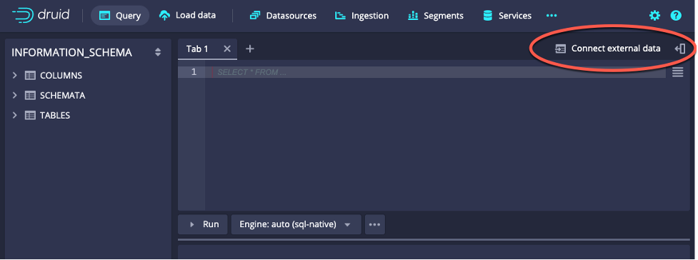
First let’s just use primary partitioning and see what the segments look like without using CLUSTERED BY. Use the “Connect external data” option in the Query view of the Druid Console:

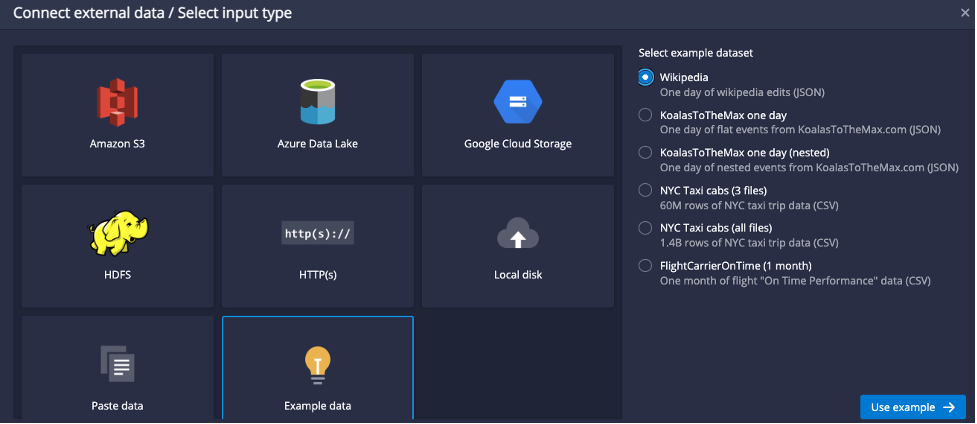
Select “Example data”, check the radio button for “Wikipedia”, and click “Use Example”:

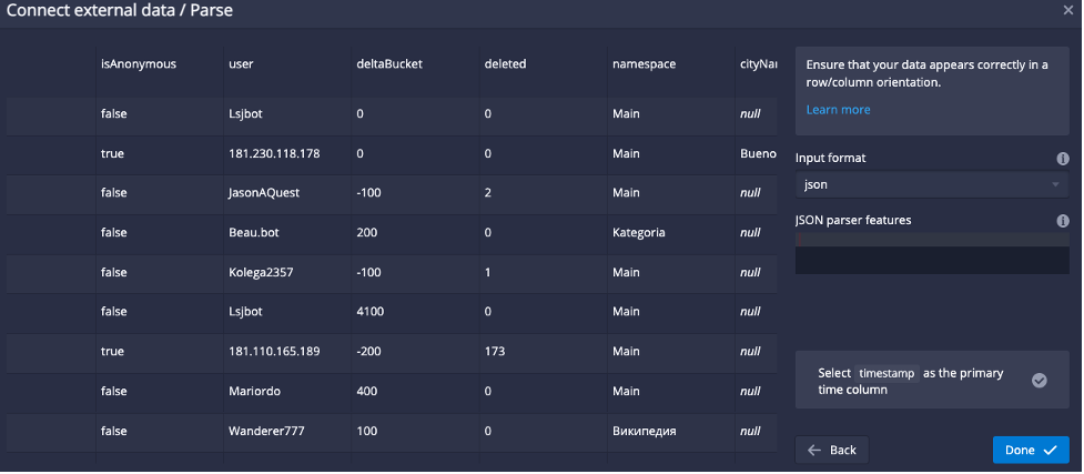
It will automatically parse a sample of the data, there’s no need to adjust it here, so just click “Done”:

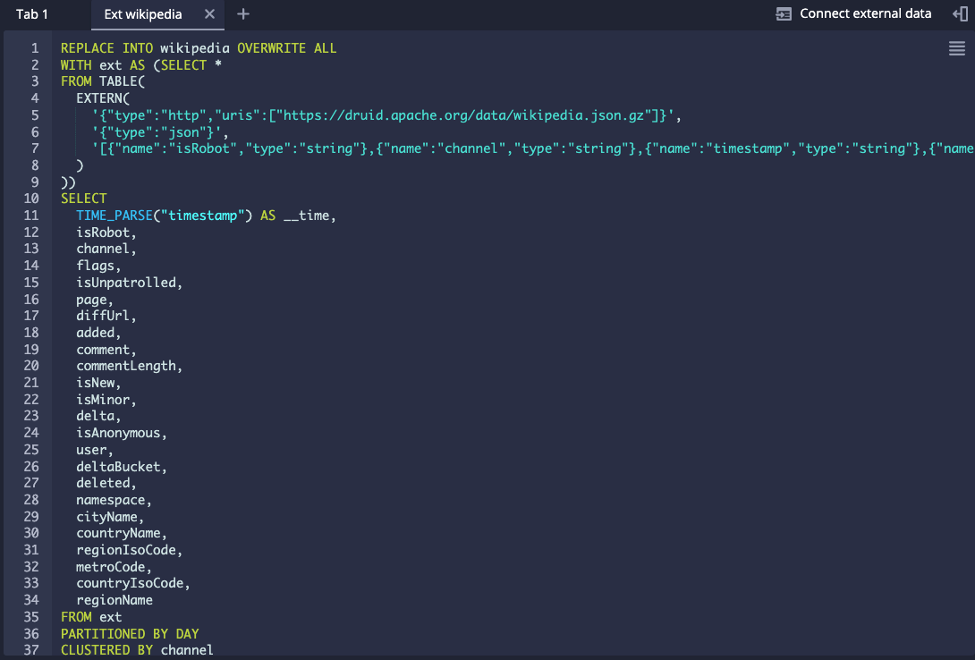
The result is a prebuilt SQL REPLACE statement with the EXTERN table function to read the external file for “Wikipedia” data:

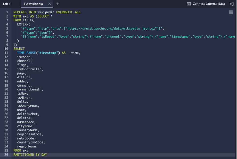
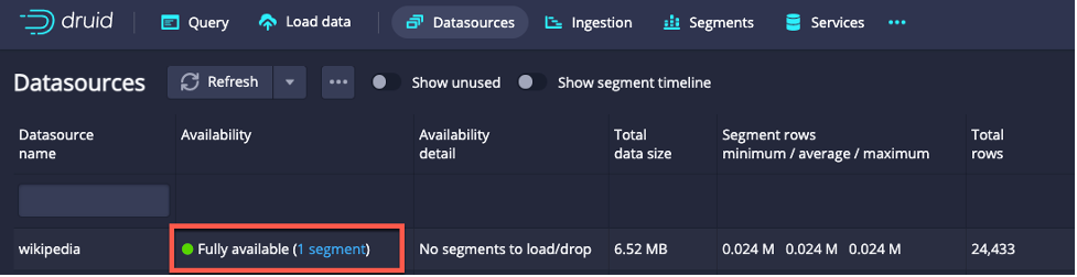
Notice that it contains the PARTITIONED BY DAY syntax at the end which sets the time chunk size to a day each. The Wikipedia data it rather small and contains only rows for a single day, so when you run this ingestion by clicking on the “Run” button, you get a single segment file, visible in the Datasources view:

For this tiny dataset we don’t really need more partitioning, even if each day contained up to a few million rows, there would be little benefit to secondary partitioning. If this is the rate of rows per day for a real-life dataset, then you’d likely benefit from using PARTITIONED BY MONTH or even coarser time partitioning in order to get a few million rows per time chunk.

But the size and set of dimensions in this data make it a good dataset to quickly experiment with, so for the remainder of this blog we will explore partitioning this dataset even though it is tiny and would normally not need it.

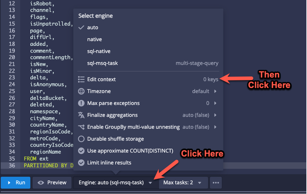
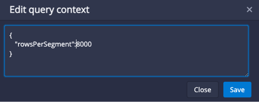
The target segment size is controlled by the Query Context parameter rowsPerSegment which you can add to through the “Edit Context” menu:

I set it to 8000, so that we can see multiple segment files and how CLUSTERED BY changes them:

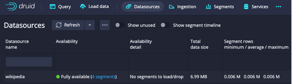
I reran the ingestion “as-is” (without CLUSTERED BY) to see how the segment files changed. In the Datasources view, you can now see four segments:

Click on the “4 segments” link to see the detail:

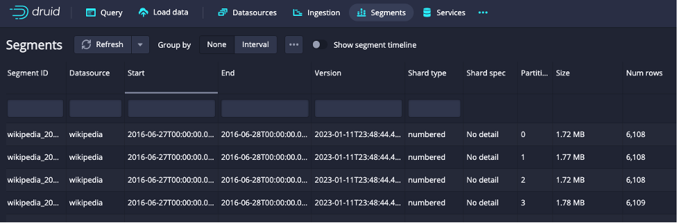
You can see that the four segments correspond to the same time chunk; the “Start” and “End” columns correspond to the same timeframe. The shard type column says “numbered” meaning that the data is not organized in any particular way, it is just split evenly into enough segments such that none exceed the rowsPerSegment value we selected.

As you can see, even without specifying a CLUSTERED BY clause, the ingestion will create partitions of a time chunk when there are more than “rowsPerSegment” rows in that interval. But given that these segments use a numbered shard type, they will all need to be processed at query time when this time interval is requested.

Secondary Partitioning with CLUSTERED BY

Segment pruning improves query response time by removing unnecessary segments from consideration. It also improves overall system efficiency by using less resources to resolve queries.

You can improve pruning by using the CLUSTERED BY clause at ingestion. The best dimensions for this purpose are the ones that will most commonly be used to filter data at query time. Let’s say you want to enable analytics for each Channel, meaning your users will almost always include a filter on that dimension. In that case, clustering by channel would be a good choice.

Using the same ingestion SQL above I added  a CLUSTERED BY clause on the “channel” dimension:

The resulting segments are still evenly split but the rows are now organized:

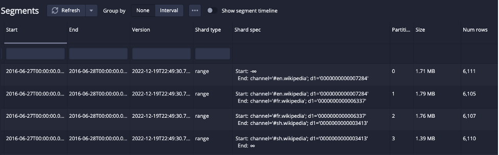
The Shard type is “ranged” and the Shard Spec shows the boundary values for the channel dimension at which it is splitting the files.  Druid automatically added another column to the range partitioning thresholds besides “channel”; it shows up here as “d1”. It is an internally calculated field that uses a hash of all the columns to create additional granularity in the boundaries in order to automatically deal with skew in the selected dimension.

Skew is the imbalance in the distribution of values of a dimension. When some values appear much more than others in the data, splitting the data along values in that dimension alone could create some segments that are much larger than others. Response times for queries are affected by this because overall query performance will be throttled by the largest segment processed. The largest segments will take longer to process causing some threads to take longer than others, this is called hotspotting. Keeping segments evenly sized will reduce or eliminate hotspotting.

Let’s review how Druid automatically dealt with skew in this example. Take a look at the counts by channel to see how skewed the dimension actually is:

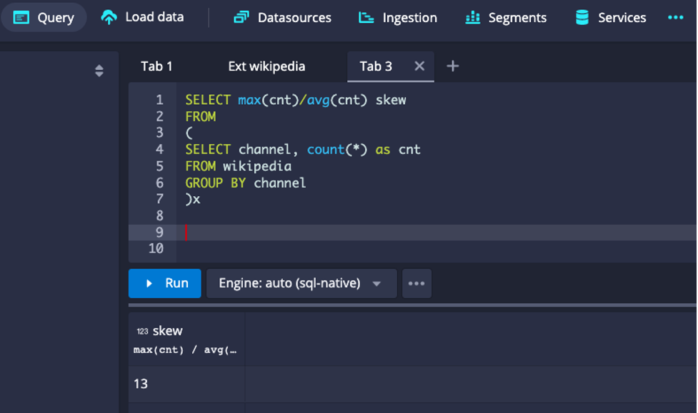
Using the ratio of the maximum row count over the average row count provides a measure of skew. In this case, it means that there is at least one value of channel that appears 13 times more often than the average. Apache Druid deals with skew by adding the hash dimension to the range partitioning dimensions in order to split the rows within the time interval evenly.

The boundaries between segments are determined within a time interval such that the generated segments each get an even number of rows.

Querying CLUSTERED Data

As stated before, using CLUSTERED BY at ingestion will improve pruning which in turn improves query performance and overall system efficiency. In this section I’ll review how pruning occurs with different query scenarios on the sample data.

At query time, if a filter on channel is used, pruning is applied such that segments without the values you are looking for are not processed. Here are a few examples of queries, and how pruning will work in each case because of the CLUSTERED BY operation above:

SELECT page, SUM(added) total_added, SUM(deleted) total_deleted

FROM wikipedia

WHERE channel = '#ca.wikipedia'

GROUP BY page

In this case only one segment will be used, since the value “#ca.wikipedia” only exists in one of the shard specs, this one:

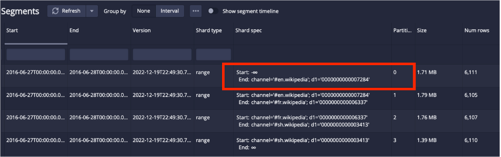
Notice that a start of negative infinity just means that all values that are less than the end boundary are included in that segment.

It supports IN list conditions such as:

SELECT page, SUM(added) total_added, SUM(deleted) total_deleted

FROM wikipedia

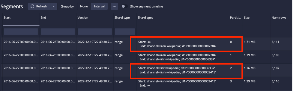
WHERE channel in ('#ca.wikipedia', '#gl.wikipedia`)

GROUP BY page

Which will process Partitions 0 and 2 that contain those two values:

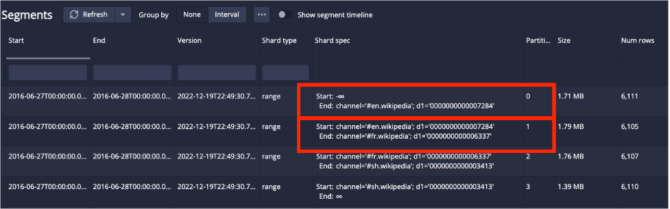
Note that filtering for values at the boundaries will use the two partitions that contain the boundary as either a Start on End value in the Shard Spec. So, querying for channel = ‘#en.wikipedia’ will require partitions 0 and 1:

It supports range conditions as well, by pruning segments that are completely outside the range filter:

SELECT page, SUM(added) total_added, SUM(deleted) total_deleted

FROM wikipedia

WHERE channel >= '#ca.wikipedia' and channel <='#de.wikipedia`

GROUP BY page

In this case, only Partition 0 is needed. The partitions that do not contain either the start or the end of the range will be pruned.

Conclusion

Using SQL to ingest data in Apache Druid is easy and powerful, it allows you to control time granularity using PARTITIONED BY, and control dimension based pruning by using the CLUSTERED BY clause. While this blog used a small dataset to show how range partitioning works, it becomes important when the number of rows within a time chunk in your dataset is larger than a few million rows (the default rowsPerSegment is set at 3 million). It makes a lot of sense to use clustering to achieve better performance of individual queries and it also drives more efficiency in the use of overall cluster resources. It is important to choose clustering dimension(s) that will be frequently used in query filter criteria such that Druid’s brokers can take the most advantage of pruning.

The fact that it deals with skew so elegantly is not just icing on the cake, although it is pretty sweet. It automatically deals with a big problem in distributed systems which frequently suffer from hotspotting when skew is not addressed. With SQL based ingestion, it is now very easy to load and organize data to achieve application analytical needs with great performance.

Learn more

• SQL Based Ingestion Clustering
• Partitioning Playlist on Youtube
• Community articles:
  • Rafał Rozpondek: Data Partitioning OptimizationJayakumar Radhakrishnan: Data Ingestion Optimization in Apache Druid
  • Hellmar Becker: Multidimensional Range Partitioning