Contributing authors: Kashif Faraz and Eric Tschetter, design partner for multi-dimension range partitioning
Reviewer: Abhishek Agarwal
Here at Imply, we run Druid clusters which churn hundreds of million rows of data every hour. And that’s only the metric data generated to monitor the actual analytical data!
For a complex system like Druid that handles enormous data loads, every component must be robust and reliable. At the same time, the system must be ever evolving.
Recently, we implemented a feature that decreased storage size by 40% while improving query speeds by 75% with absolutely no loss in data fidelity. Here we discuss the twists and tweaks of an integral cog of the Druid machinery which made these improvements possible: partitioning.
(TL;DR: If you are a person of few words, please refer to the table at the end to choose the best partitioning scheme for your use cases.)
The partitioning motivation
Anyone who works with data is already familiar with techniques such as partitioning, sharding and bucketing as a means to improve performance. But for the joy of listing things, let’s rehash some of the potential benefits partitioning could offer in Druid:
- Parallelism: Multiple processes can operate on different portions of data simultaneously.
- Distributed storage: Data can be spread across several data servers thus allowing even commodity hardware to meet memory and disk requirements.
- Improved I/O management: Reasonably sized partitions make reading from/writing to disk easier and transmission over network less prone to failure.
- Granular replication: With the same factor, say 2, replication at the partition level allows better fault tolerance than replication of unpartitioned data as a whole.
Perhaps we needed that refresher after all. It reminds us that partitioning is not a luxury, but rather a necessity for a scalable database system. Now let’s take a moment to consider what kind of a partitioning scheme would actually meet our needs.
The paradoxical partition
‘Spread out’ for Write
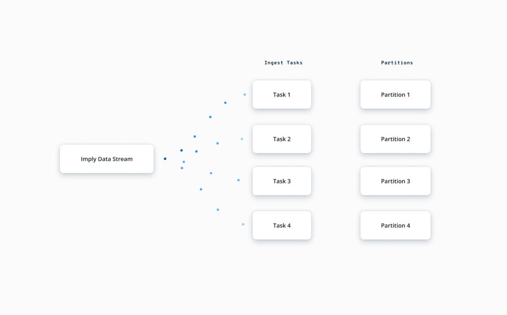
Streaming ingestion is a popular method of loading data into Druid. To ensure rapid event processing and to avoid lag, the streaming pipeline should organise data in a write-optimized manner that minimizes hot-spots. This would mean spreading out the incoming data across several partitions to evenly distribute the ingestion workload among multiple processes and servers.
‘Group up’ for Read
Druid loads the absolute minimum amount of data necessary for a query to optimize performance. It uses indexes and other metadata to aggressively prune out rows which are not needed for a query.
For example, imagine we have data for a whole year with 365 partitions, one for each day. When querying for the first week of January, we need to look at only 7 partitions and ignore the remaining 358. This would help us save significantly on compute resources and/or query time. But if the data for a single day were spread across many partitions, this strategy would be less effective. Simply put, we must partition by time to actually benefit time-based queries.
The practice of storing similar data together is referred to as ‘data locality’. The similarity can be on the basis of the values of one or more columns (typically dimensions). Along with query performance, locality also helps in reducing disk footprint as co-locating similar data allows for better compression.
Hot-spot or not?
It is evident that both ingestion and queries can benefit through partitioning but they have contradictory requirements. While the former requires eliminating hot-spots by spreading data out, the latter benefits from similar data being stored together, effectively creating hot-spots.
A timely solution
Despite the differences between read and write operations, the time dimension plays a key role in both of them. This is only to be expected since all event-oriented data and the insights drawn from it are more meaningful when considered over a time duration. Even simple questions like “What is the total number of users?”, “What is the increase in sales?” are more meaningful when you add the words “today”, “since last month”, or “over all time” to them.
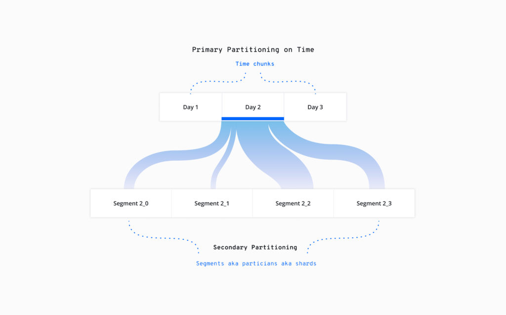
Thus, Druid always partitions data by the timestamp dimension at a chosen segment granularity. For example, choosing a granularity of ‘DAY’ would divide the data timeline into several chunks, each containing the whole data for a day.
Such a time-based partitioning certainly benefits queries with a time filter. However, it might not work as well for write-time parallelism. This is because consecutive events in the input data stream, with adjacent timestamps, would be written to the same partition. Another concern is that as data grows and you start seeing billions of events an hour, even the finest time granularities will not yield partitions of a manageable size.
The solution is secondary partitioning to further divide each of the time chunks into smaller partitions (aka segments). This enables us to retain write-time parallelism and create appropriately-sized partitions while continuing to benefit time-based queries. Secondary partitioning can also create more opportunities for pruning out unnecessary rows based on column filters in a query.
Re-organization by auto-compaction
Partitioning by time takes us only half of the way because we are still left with the question, how should the secondary partitioning work? Should it spread out incoming data in favour of write-time speed or should it group similar data together to improve read-time performances? Unfortunately, these requirements are mutually exclusive and we cannot have a single data layout that satisfies both of them.
The good news is that Druid is a WORM (write once read many) system. We need to optimize for write only during ingestion as all later operations will only be read. This means that data can be ingested from the stream in a write-optimized manner which spreads it out in favour of parallelism. After the data is old enough to have no more writes, Druid can reorganize it in favor of data locality.
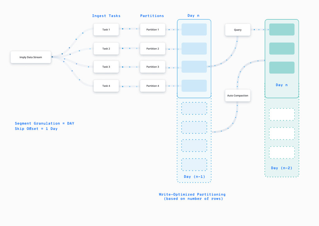
This convenient process of rearranging data in Druid is known as ‘compaction’, so called because the resulting column-based partitioning allows for rollup as well as greater compression. You can schedule compaction to run periodically with configurations defined to attain the best data layout for your querying use cases.
Row distribution
Now that compaction allows us to choose different partitioning schemes for ingest-time and query-time, let’s find the best candidates for the two. Until recently, Druid supported the following secondary partitioning schemes:
- Dynamic: The default scheme, which creates a new partition after every N rows. It provides no data locality but creates uniformly sized partitions.
- Hashed: A dimension-based scheme, which creates partitions based on the hashed value of chosen partition dimensions. It offers low data locality and creates more or less uniform partitions.
- Single-Dim: A dimension-based scheme, which uses the range of a single dimension to create partitions. While it boasts of a high data locality, it can often create partitions that are much larger than the target size.
Let’s have a closer look at each scheme by applying it to the following sample dataset from a typical e-commerce website.
| id | category | sub_category | num_items | checkout_price |
|---|---|---|---|---|
| 1 | electronics | tablet | 1 | 107 |
| 2 | apparel | kids | 3 | 316 |
| 3 | electronics | phone | 1 | 405 |
| 4 | furniture | table | 1 | 126 |
| 5 | apparel | shirts | 3 | 352 |
| 6 | electronics | laptop | 1 | 700 |
| 7 | kitchen | cutlery | 10 | 525 |
| 8 | electronics | laptop | 1 | 950 |
Dynamic Partitioning
With a target partition size of 2 rows each, dynamic partitioning of this dataset looks something like this:
| id | category | sub_category | partition number |
|---|---|---|---|
| 1 | electronics | tablet | 0 |
| 2 | apparel | kids | 0 |
| 3 | electronics | phone | 1 |
| 4 | furniture | table | 1 |
| 5 | apparel | shirts | 2 |
| 6 | electronics | laptop | 2 |
| 7 | kitchen | cutlery | 3 |
| 8 | electronics | laptop | 3 |
By definition, the dynamic scheme creates partitions of size as close as possible to the target size. It is best suited for write-time operations as incoming data is written to uniformly sized partitions without the need to shuffle rows. The primary drawback is that dynamic partitioning doesn’t care about data organization at all. Note that each of the 4 partitions has a row for ‘electronics’. There is no data locality because the column values play no role in determining the partitions.
Hashed Partitioning
Hashed partitioning allows us to partition on any number of dimensions, so let’s use both category and sub_category. The number of partitions is determined by the given target size.
Num Partitions = Num Rows / Target Size = 8 / 2 = 4Possible partition numbers = {0, 1, 2, 3}
We need a hashing function to map the dimension values to a valid partition number. While the function used in practice is a 32-bit Murmur 3 Hash, let’s define a simpler one here that we can actually follow:
Partition Number = (length(category) + length(sub_category)) % 4i.e. the partition number is the total length of category and sub_category columns taken as a modulo of 4.
| id | category | sub_category | total length | partition mumber |
| 1 | electronics | tablet | 17 | 1 |
| 2 | apparel | kids | 11 | 3 |
| 3 | electronics | phone | 16 | 0 |
| 4 | furniture | table | 14 | 2 |
| 5 | apparel | shirts | 13 | 1 |
| 6 | electronics | laptop | 17 | 1 |
| 7 | kitchen | cutlery | 14 | 2 |
| 8 | electronics | laptop | 17 | 1 |
The distribution above demonstrates the following:
- There is some data locality because all rows for (‘electronics’, ‘laptop’) are assigned to partition 1. With hashed partitioning, rows with the same combination of dimension values always end up in the same partition. This implies that if a query were only looking for rows with category=‘electronics’ AND sub_category=‘laptop’, we could safely ignore all the other partitions.
- The data locality is not perfect because rows for other ‘electronics’ items have ended up in other partitions.
- The distribution is not as uniform as dynamic partitioning: one segment has 4 rows and one has only a single row
- It is rather difficult to predict the final layout due to the complexity introduced by the hashing function (even a simple one).
Single-Dim Range Partitioning
Let’s partition our sample data on the dimension category with the same target partition size of 2 rows each. To determine the distribution, we must first identify the range of the partitioning dimension and then create boundaries at appropriate intervals. The distribution looks something like this:
| id | category (sorted) | sub_category | partition number |
|---|---|---|---|
| 2 | apparel | kids | 0 |
| 5 | apparel | shirts | 0 |
| 1 | electronics | tablet | 1 (boundary) |
| 3 | electronics | phone | 1 |
| 6 | electronics | laptop | 1 |
| 8 | electronics | laptop | 1 |
| 4 | furniture | table | 2 (boundary) |
| 7 | kitchen | cutlery | 2 |
The above layout demonstrates great locality because all the rows for ‘electronics’ are in partition 1. But at the same time, that partition has 4 rows: twice the target size! This is because with single-dim, all rows for a given value of the partitioning dimension (here category) always go to the same partition. So while querying for rows with say category=‘furniture’ or category=‘kitchen’, we would need to look only at partition 2.
Multi-dimension generalization
Single-dim partitioning offers a high data locality which benefits both query performance and storage efficiency. But there are two primary challenges with using single-dim:
- Only one partition dimension: It is difficult to choose a single dimension that is likely to satisfy all the requirements of partitioning, i.e. improve locality, boost query perf, etc.
- Uneven partition sizes: In the example above, we saw that partitioning on a single dimension can result in uneven partitions as real-world data is often skewed.
If we could somehow mitigate these drawbacks, single-dim partitioning could very well become the best read-time strategy. Driven by this lucrative possibility, we began to investigate the effects of including more dimensions in range partitioning. For example, if we were to partition on the ranges of the tuple (category, sub_category) instead of just category, the distribution for the above dataset would be as follows:
| id | category (sorted) | sub_category (sorted with category) | partition number |
|---|---|---|---|
| 2 | apparel | kids | 0 |
| 5 | apparel | shirts | 0 |
| 6 | electronics | laptop | 1 (boundary) |
| 8 | electronics | laptop | 1 |
| 3 | electronics | phone | 2 (boundary) |
| 1 | electronics | tablet | 2 |
| 4 | furniture | table | 3 (boundary) |
| 7 | kitchen | cutlery | 3 |
We can see that the partitions are more evenly sized as compared to single-dim. Adding sub_category allows the ranges of both the dimensions to help determine the partition boundaries. So the rows for ‘electronics’ can now be split across two partitions without compromising on data locality.
Safe experimentation
Encouraged by these observations and some proof of concept work, we ventured a little deeper into the world of multiple dimensions – a Druid multiverse if you will. We implemented the prototype of a partitioning scheme that could work across any number of dimensions, thus creating multi-dimension range partitioning aka ‘multi-dim’.
Imply Clarity is an APM product which allows users to monitor their Druid clusters’ operational health. It is powered by a large Druid deployment itself and provides deep visibility into query performances and data flow. Built specifically for Druid, Clarity makes it very easy to pin-point performance bottlenecks and hot-spots on Druid clusters.
Given the huge data load churned by the Druid cluster for Clarity, we found it to be the perfect avenue for further experimentation. What better way to validate our theories than to test them on production data (with supervision, of course)? With a solid 75% decrease in query times and a 40% decrease in storage size over un-compacted data, multi-dim proved itself to be the best read-time partitioning scheme for most, if not all use cases.
A comparative conclusion
Druid always partitions data by the timestamp dimension to benefit time-based analytical queries. A secondary partitioning is needed to further break down the time chunks into manageable partition sizes.
Based on the observations above, we can all agree that ‘dynamic’ is the best scheme for write-time partitioning, especially with streaming ingestion. A periodic auto-compaction can then reorganize the data with a suitable read-time partitioning.
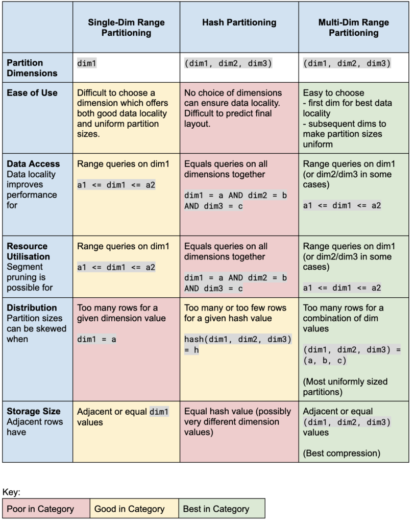
To help you choose the best scheme for read-time, we have compiled a summary of all the options now available in Druid. Here’s a hint, go for the green one!
Too good to be kept a secret, multi-dim will soon be available in Apache Druid 0.23 for everyone to use. In the meantime, it already comes packaged with Imply 2021.12 (refer to docs here). Feel free to try it out on any dataset of your choice (even prod). Stay tuned for our upcoming blog where we take you on the journey of our own multidimensional adventures!
 Architecture
 Deployment
 Ingestion
 Modeling
 Operations
 Development


