Learn how to achieve sub-second responses with Apache Druid

Introduction

Data-driven applications and dashboards place performance and scalability demands on databases. Just one poorly designed query can make or break the user’s experience, as can the high numbers of queries per second that internet-facing apps and dashboards generate.

Apache Druid® was built for just this scenario – with the promise that its data format, architecture, and massively-parallelised operations help us to deliver on the levels of performance needed for real-time exploration.

The late Carl Sagan tells us that, “if you want to make an apple pie from scratch, you must first invent the universe.” If you want to have a performant data application, you must first understand how the query engine powering your application works – from the ground up. Any discussion I’ve had about query performance in Apache Druid has inevitably led to a discussion about data modeling and layout. When I’ve seen people ingesting data just to get the job done (treating Druid like a data lake, for example) they ignore this important relationship about how these two things influence and affect each other.

In this article, I’ll examine this interplay between data modeling and query performance in Apache Druid, and cover the four go-to data modeling techniques that you can apply at ingestion time:

Rollup (GROUP BY)
Sharding (PARTITIONED BY and CLUSTERED BY)
Sorting
Indexing

Unlocking Druid Performance

Take this diagram of how clients submit queries to Druid.

At the top, clients submit queries to the Broker (1). From there, the queries fan-out (2), distributing the queries to data processes (Historicals and Indexers / Peons). Each one handles its piece of the query (3) and returns the results to the Broker via a fan-in (4). The Broker merges the results (5) and serves them to the user.

Examining this in greater detail will inform your data modeling decisions giving you the tools to understand and improve performance. This Query Stack diagram helps us understand how Druid returns results:

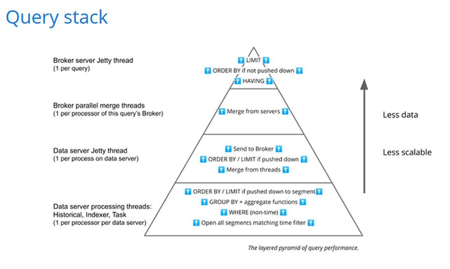
Queries on tables execute with a fan-out / fan-in approach which is also called a scatter / gather approach. The bottom two layers of the diagram are data process activities, the top two are Broker activities. The fan-in mechanism happens in between these two halves, connecting the Broker and data servers.

The diagram is shaped this way because it illustrates the level of parallelism involved in each stage. The bottom layer is more scalable because it is where the highest parallelism is achieved. But as processing moves up through the layers, there is progressively less parallelism involved. The impact is that queries that use the fan-in / fan-out execution pattern perform best when the volume of data reduces as processing moves up through the stages.

With that in mind, let’s look at each of the stages and how the infrastructure we provide to Druid is utilized.

Submitting the Query

The first step in query processing happens on the Broker.

It can distribute queries into different priority queues, this is called Query Laning. It enables you to manage mixed workloads with Druid, with fast queries getting the resources they need to be fast while keeping longer-running, more resource intensive queries in check. Read all about that in Kyle Hoondert’s great article Query Prioritization in Apache Druid.

Query Planning and Fan-Out

The Broker parses the request and figures out which segments of data are needed to respond to the request.

This is why the WHERE clause __time condition in your query is so important. Druid maintains an in-memory index of the table timeline, and the Broker uses this to find which data processes contain copies of individual segments that cover the requested part of the timeline.

If the data source uses secondary partitioning on other dimensions and you include a filter on those dimensions in the WHERE clause, the Broker uses this information (which is also in the global index) to further prune the list of relevant segments to process.

Check out my video series on secondary partitioning where I describe what goes on at ingestion time to generate the partitions and how each partitioning strategy helps prune at query time.

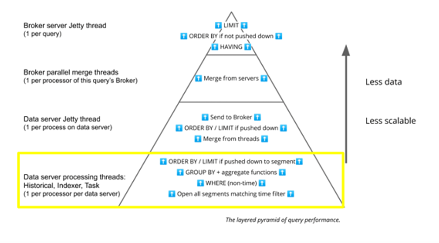
Data Server Processing Threads

Once the Broker has identified the data it needs, it issues requests to the corresponding data processes that have those segments available. Each data process executes its portion of the query: streaming ingestion tasks (Peon / Indexer) process recently consumed data, Historicals process already ingested data.

Starting at the bottom layer of the diagram, we can now turn to the individual processing threads on those Historicals and Indexers / Peons involved in executing the query plan.

Historicals

Each thread works on one segment at a time.

The thread evaluates the WHERE clause to apply filters, including trimming __time even further, and examines the filtering columns’ dictionaries and indexes to find the relevant rows within each segment.

For more complex WHERE clauses the thread uses bitmaps from multiple index entries across different columns and bitwise operations among them to find the right rows.

If the query uses GROUP BY, the thread then performs local aggregation on the selected rows.

Depending on the query pattern, the results may be ORDERed and LIMITed at this point.

Zoom out a little, and you can visualize how this is happening in parallel across multiple threads on multiple Historicals. When a table is made up of too many small segments it can generate management overhead because it will use many more threads to process many more segment files. Conversely, tables that have segments that are too large – even just one or two – cause delays in single threads that impact the overall parallel operation.

Read more about Segment size optimization in the official documentation, where you’ll see it’s best practice to balance segment sizes, and to keep them large enough to be efficient (approximately 5 million rows per segment with sizes in the 500-700 MB range).

Streaming Ingestion Tasks

When the query’s __time filter covers time intervals that streaming ingestion tasks are working on, the Broker submits the request to all the tasks involved.

Each task is in charge of certain shards of the incoming stream (e.g. a set of partitions in Kafka). Each task holds the rows associated with its shards in memory until the buffer is deemed full, at which time it spills the rows to disk into files in what’s called an “intermediate persist”.

When a query request arrives, the task merges the in-memory row buffer with any intermediate persists it has accumulated and resolves its portion of the query on that data. Just like in Historicals, the task filters and aggregates its local data, and might apply ORDERs and LIMITs before finally sending its results to the Broker.

Zooming Out

You can now see that there’s a high degree of parallelism at this stage. This bottom processing layer is constrained only by the number of threads available. Increasing resources here will likely help in query performance and in dealing with higher concurrency. That means providing enough cores to handle enough segments to support the parallelisation – and making sure that your segments are the right size.

Data Server Jetty Thread

Moving up the Query Stack diagram, there’s a single Jetty thread per query in each data process that takes the results from the individual segments and merges them into a single result set that it can percolate up to the next level – the Broker.

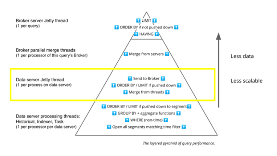
The Jetty thread accumulates all the data from the segment processing threads and does the final merge, filter, aggregation, ORDER BY, and LIMIT as needed.

Here, the opportunity for parallelism is reduced. Only one thread for each query is activated to do this work in each data process: one per Historical, one per streaming ingestion task.

You need to consider how much data the segment-processing threads are returning to this merging thread. For example, a GROUP BY on a high-cardinality dimension can cause a bottleneck, as would a SELECT * with many columns or a query without enough filtering in the WHERE clause.

Broker Parallel Merge Threads

The next step sees the Broker merge the partial results from each of the data processes.

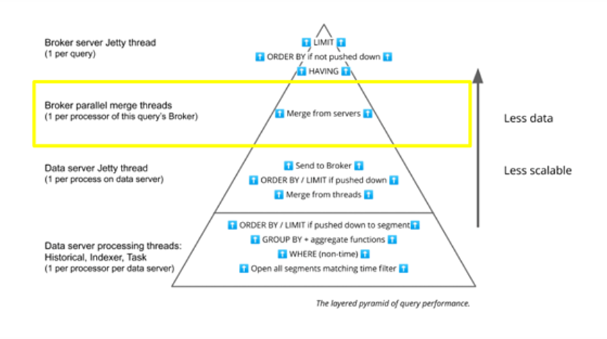
At this point, a Druid query does not scale out – it is located in one specific Broker. Imagine you have Brokers that are 16 cores each, and you have 10 of them. Even with 160 processors at your disposal, only 16 can be used for this merge stage as that’s where this query is being governed.

Monitoring core utilization on individual Brokers when queries execute is key here. You should have enough capacity per Broker to merge results from across your data servers at query time for many concurrent requests.

Broker Server Jetty Thread

Finally, at the very top, the Broker server Jetty thread completes the operation that evaluates the final LIMIT, ORDER BY, or HAVING clauses on the merged result.

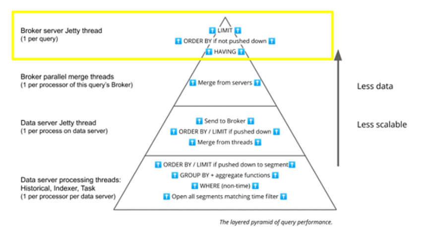
This query step is single threaded, so for best performance we don’t want to have too much data or too many operations taking place here as these will rapidly cause a bottleneck.

As an example of the complex interplay between data modeling and query performance, it is much more efficient to push the LIMIT and ORDER BY down to the data server processing threads where query performance can scale better. Druid does this automatically for LIMIT clauses that run with the native Scan or TopN query types, and for ORDER BY clauses that run with native GroupBy query types. Adding LIMIT and/or ORDER BY clauses that push down to data servers is a great technique to boost performance in Druid.

The Query Stack in Action

Let’s dig deeper into the bottom layer of the Query Stack to see how to split things up and optimize for performance.

One way to think about how Druid operates is that the query fans out to a bunch of segments, and then the response fans-in. This is significant because we see lots of examples where queries bottleneck at that bottom layer. It’s easy to see that this is what is happening when queries are running and data server CPUs are pegged at 100%. That’s a clear indicator that that bottom layer is where the action is happening, and this is a typical Druid experience. Of course, any layer could be a bottleneck; the best way to identify the bottleneck is with flame graphs.

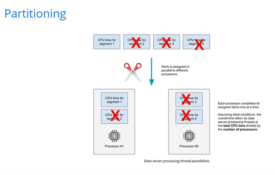
At the bottom layer there’s a set amount of CPU processing (or CPU time) that needs to happen on each segment to execute the query, i.e. segment one is going to take a certain amount of time and segment two will take a certain amount of time. These times are fixed for a given data set and a given query. A query on segment number one might take 400 milliseconds of CPU time. It’s not possible to change how fast that runs, but it is possible to add more processors and increase parallelism. You can keep adding processors until the number of processors equals the number of segments, and at that point adding more doesn’t decrease the amount of time needed because we can’t split a segment between multiple processors.

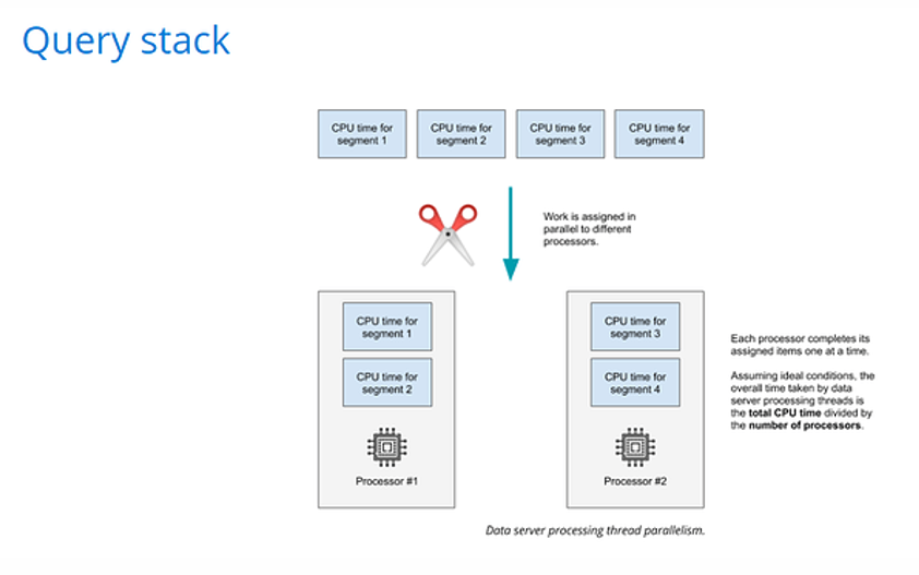
Druid processes segments in parallel across the available CPUs / threads. The total processing time that the bottom layer takes to process a query is therefore roughly the total CPU time needed for all segments divided by the number of processors available.

This is the beginning of a formula that will help us understand query performance…

Performance Algebra

It’s possible to break down different factors that come into play in determining query performance. Here’s a model for overall query performance that considers most of the factors. After we define it, we’ll connect the various pieces to the data modeling and query techniques that can help improve each factor.

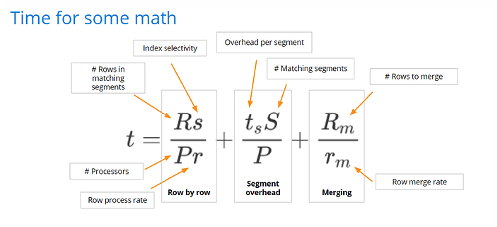
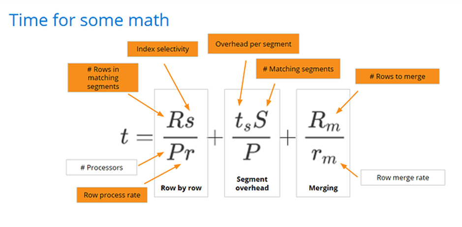
t is an estimate of the time a query takes to complete, it has three major components:

Rs/Pr = Total row level processing time

R – (rows) total number of rows in the selected segments

s – (%) index selectivity – percentage or rows filtered

P – (CPUs) number of CPUs available for processing

r – (rows / cpu second) row processing rate

t_sS/P = Segment overhead

t_s – (cpu seconds) segment processing overhead

S – (#) number of matching segments

P – (# CPUs) number of CPUs available for processing

R_m/r_m = Merging

R_m – (rows) total number of rows to merge

r_m – (rows / cpu second) number of rows merged per second

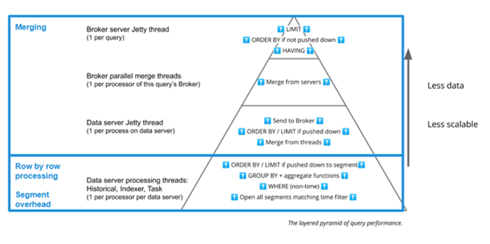
Row by row processing and segment overhead take place in the bottom layer of the Query Stack, while merging takes place in the top three layers.

Focusing on row by row processing, one way to think about it is that Druid will need to use a certain amount of CPU time to complete the request, and dividing that by the number of available CPUs, we can estimate the duration of the bottom layer of the Query Stack.

The term Rs over r is the amount of CPU time needed to process all the segments. Dividing that by P given that processing occurs in parallel, results in the time estimate for the first phase.

s is the selectivity of the filters in the query which can have significant impact on overall query time. If a query WHERE clause returns half the rows, index selectivity is one-half (0.5). Alternatively, if a query is not filtered, then index selectivity is equal to one (1.0). Reducing the number of rows to process will have a direct effect on performance.

Let’s work through an example: say we have 2 years of sales transactions for a chain of 1000 stores which on average have 100k transactions each per day. If we create daily segments that each have about 5 million rows, we will end up with about 1000 * 100k / 5 million rows per segment = 20 segments per day.

If we query one week of data, the total number of rows within matching segments would be R = 700 million rows split over 140 segments. When filtering on a single store, index selectivity will be 1/1000 = 0.001 resulting in only 700k rows.

If the row processing rate is 10 million rows per cpu second then total CPU time will be:

Without filter: 700 m / 10 m = 70 cpu seconds
With single store filter: 700 k / 10 m = 0.070 cpu seconds

Both queries can be fast given enough CPUs. With P=70 cpus, the first query can be done in 1 second and given that we are dealing with 140 segments, each CPU can process two segments in parallel. We could make it even faster with up to P=140 CPUs to resolve the query in 0.5 seconds. More CPUs than P=140 CPUs would not make the query any faster, given that each segment is processed by one thread which runs on one CPU.

With the filtered query, there is a lot less data to process, so the query will be faster. Using filters is a great way of speeding up queries in Druid. But keep in mind that the query will still need to process 140 segments, and that’s where the next term of the equation comes into play.

The segment overhead per segment t_sis a result of how the data server processes the query, where each thread must process a segment at a time. Per segment processing, t_s is multiplied by the number of segments S that hold the data for the query giving a total cpu seconds needed, divided by the number of CPUs P. However, t_sand P can only be affected by changing the composition of the cluster with faster CPUs and more CPUs. You can see why we love compaction in Druid. Compaction can reduce the number of segments to make this term smaller. More generally speaking, segment size optimization is a best practice that will help optimize this term.

The last portion of the equation is merging, where the number of resulting rows from the row processing phase R_mwill need to be merged. Notice that this is only true in an aggregation query, where row merging is necessary to calculate final grouped results. We determine the row merge rate r_m mostly by the query server size; the query server is the one running the Broker service. The more powerful the server, the larger the row merge rate. Therefore the merging component of the equation has less impact. On the other hand, the number of rows to merge R_mis based on the cardinality of the grouping dimensions, with more rows to merge giving the merging component of the equation more impact.

Data Modelling and Performance

Now let’s consider the connection between data modeling and performance. Returning to our equation, note that some of the variables are now orange. The orange variables are ones that we can affect with data modeling.

The only things we can’t affect through modeling are the row merge rate, which we saw earlier is heavily dependent on query server size, and the number of CPUs. We can affect everything else in this performance equation by optimizing data modeling with Druid. There are four major data modeling techniques used to improve performance in Druid: rollup, partitioning, sorting and indexes.

Rollup

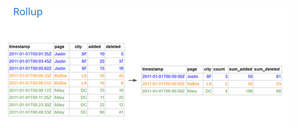
Rollup in Druid is a process of summarization, an optional feature that serves to reduce the row count through pre-aggregation. Rollup at ingestion time, treats columns as either dimensions or metrics. It aggregates metrics by grouping on time and the unique combinations of dimension values. At query time, users may apply further aggregation along a subset of dimensions and do other metric calculations. The general idea is to do partial aggregation at ingestion to the level of granularity that is useful for querying. This is one of the ways that Druid accelerates query response times.

Rollup can be applied during both real-time ingestion or batch ingestion. For batch ingestion use SQL-based ingestion which allows you to specify the aggregation as a simple insert or replace statement with a SELECT using GROUP BY in the form:

INSERT/REPLACE INTO <table> 
SELECT FLOOR(“timestamp” TO HOUR) AS __time, # primary time column
      page, city,                            # dimensions 
      COUNT(*) as “count”,                   # metrics
      SUM( added) as “sum_added”,            # metrics
      SUM( deleted) as “sum_deleted”         # metrics
FROM TABLE (EXTERN ( … ) )                   # input source
GROUP BY  1,2,3
PARTITIONED BY DAY                      # time partitioning
CLUSTERED BY page                       # 2ndary partitioning

Truncating Time

Note that when applying rollup, it is common to truncate the primary time column to a level that is useful for users of this data. With native or real-time ingestion this is called the query granularity. When using SQL-based ingestion, it is a transformation of the input “timestamp” by truncating it to the desired time unit. Many times, hourly aggregation or minute by minute aggregation is more than enough granularity to achieve users’ goals.

Grouping Cardinality

Depending on the peculiarities of your data, rollup may do absolutely nothing, which may occur if there’s some combination of dimensions in your data set that is unique in some way. For example, this could happen with unique IDs in the data set, or an IoT data set that has only one data point per minute, and you’re grouping on minute and sensor. In either of these examples, the data set is such that no actual grouping occurs so the grouping does not improve performance. So, we see that rollup may result in no performance improvement or may yield great performance improvement, providing a 20 to 40 times reduction in data size and commensurate 20 to 40 times increase in performance. But even a bit of rollup at ingestion will help.

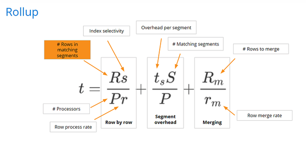
Rollup effectively decreases the number of rows R in the matching segment. It reduces the number of rows in the data source, and therefore the number of rows across all the segments that match a query.

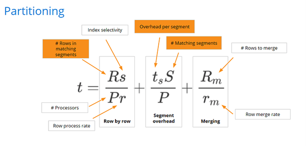
Secondary Partitioning (CLUSTERED BY)

At query time, filtering on the columns used for secondary partitioning will likely reduce the number of segments Druid needs. Secondary partitioning is configured in the tuningConfig section of native batch inserts or compaction jobs. We can also specify secondary partitioning using the CLUSTERED BY clause in SQL Based Ingestion.

Partitioning matters most for situations where users consistently filter on the same selective column. A canonical example is a multi-tenant situation where there is a column for customer ID, and users are always filtering by customer ID so that the users only see their own data.

Partitioning can significantly improve Druid performance because the system can now process a subset of segments within the filtered time frame. Note that not all queries will improve in this fashion. Only those that filter on the partitioning dimension(s) will benefit.

Looking at our equation, partitioning and filtering on the partitioning column affects the number of rows in matching segments and the number of matching segments. Fewer segments will match the query filter, and less segments means less rows.

Sorting

Every segment partition stores its row data pre-sorted. The sort order of the rows within a segment file will always follow the order in which the columns are ingested, sorting first on the primary __time dimension, followed by all columns as specified either in the SQL-based ingestion SELECT query, or in the dimensionSpec when using native ingestion.

Given the same values of __time, secondary sorting will follow with the next dimensions in the list. If you use queryGranularity in native batch ingestion or truncate time using an expression (i.e. FLOOR( “input_timestamp” TO MINUTE) ) in SQL-based ingestion, you can increase the locality of values in the dimensions that follow __time because there will likely be more rows with the same time value. This improves compression which in turn improves I/O performance.

Given that partitioning already organizes segments into ranges of values for a given dimension, placing that dimension first after __time is likely to increase locality of the same values. This is why we recommend listing the partitioning/clustering dimensions first which will drive primary sorting of the segment.

Let’s look at our equation to see why sorting helps.

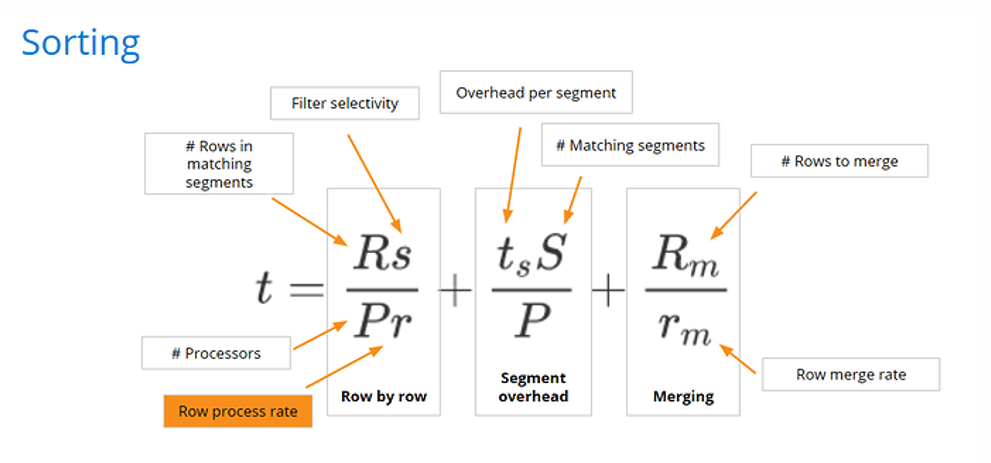
Sorting improves the row process rate so we can process rows faster. It’s much harder to scan through jumbled chunks, decompressing and compressing them, because they’re out of order. The combination of partitioning and sorting is very valuable towards improving Druid query performance. Partitioning speeds up three variables in our performance equation and sorting adds another variable to improve. Together, partitioning and sorting optimize the bulk of our performance equation.

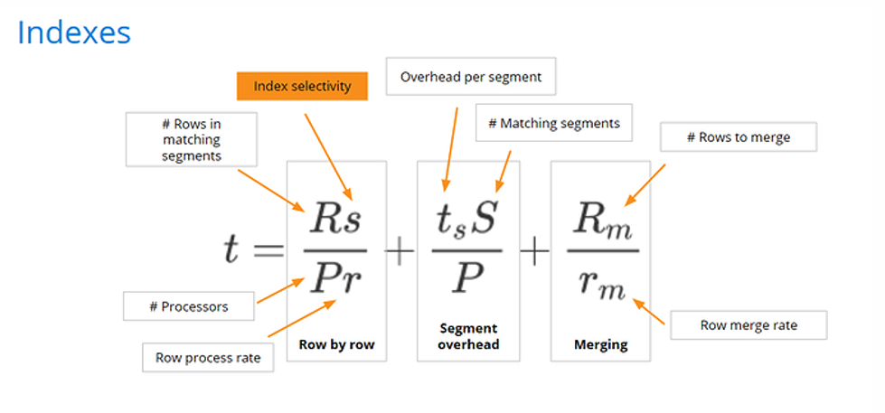
Indexing

Today, Druid indexes string columns and numeric fields within Nested Columns. The Apache Druid project is adding first level numeric column indexes soon. As we saw when discussing index selectivity, filtering on columns with indexes helps query performance. This means that we may further optimize performance by ingesting first level numeric columns as strings. This is a little bit counterintuitive because usually with data systems for best performance it’s best to model things in their most natural type. This happens to be an exception, and it is only temporary.

Indexes work by first looking up the filter value in the column’s dictionary, which is always sorted, and from there looking at the same position in the index where both reverse lookup and bitmaps are stored. Reverse lookup provides the row numbers within the segment that contain the value. If the filter condition is on multiple columns, bitmaps are used with bitwise operations to find the rows of interest.

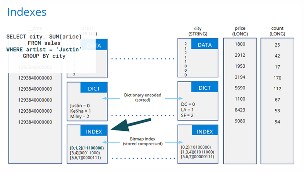
Imagine that your data set includes a field for a number that users always filter on, e.g., customer ID. Users are always filtering on customer ID, and never running any aggregations that would require the field to be numerical. In this case, it’s beneficial to store the customer ID field as a string so it gets an index.

In the future, Druid will get indexes on numeric columns, but until then, you can help boost query performance with this powerful technique. In our performance equation, we reduce index selectivity s.

A Few More Thoughts on Modeling with Druid

We need to provide enough flexibility in our model such that Druid can calculate the metrics and statistics at the level of granularity that users need. But having a bias toward aggregation at ingestion and toward solving queries with more aggregate tables will serve us well. Overall, while more tables may use more storage and more CPU at ingestion, it will reduce the CPU needed to process queries. Ingestion occurs once, queries will occur many more times on the same data. Reducing the CPU cost of the query side will use resources more efficiently and enable higher concurrency.

Some very successful implementations of Druid ingest from a single stream of events into multiple tables. They use tables with different time granularities and varying levels of aggregation. We need to think in terms of what analytics are needed and along which dimensions.

We may want to keep a detailed data table, but we should design the applications that query it to use enough filtering to limit the Rows and Segments per query. It’ll be good to have the detailed data around as a source for backfill when developing new functionality or changing aggregation and partitioning strategies. The detail table should be partitioned on the dimensions that are used for filtering those detailed queries to reduce the segment count needed to get the results.

We should use other tables with more aggregation for subsets of functionality when the query workload and its performance expectations warrant it. We should look for opportunities to use approximation functions to remove high cardinality items. Take a user_id column from event data on a mobile app used by millions of users. Perhaps all you need are distinct counts and / or quantile statistics on user activity of the distinct values of user_id which has very high cardinality. Removing user_id in a rollup ingestion will help reduce R. Evaluate whether an approximation with enough accuracy is sufficient for the use case and, if so, replace the column with the appropriate approximation function.

We’ve talked about how secondary partitioning in combination with filters on the dimensions will reduce R and S. Also consider that with secondary partitioning you’ll reduce R_m when grouping on the partitioning dimensions. By partitioning on the dimensions that are commonly grouped on, you pre-organize the data so that it is more likely that the aggregate result for a given grouping value is within one or just a few segments. This improves processing efficiency. Consider a query with GROUP BY that includes the partitioning dimensions. The partial aggregation at the bottom layer of the Query Stack where there is higher parallelism will produce less results, effectively doing more merging sooner. The results are naturally reduced as rows with the same value for the grouping dimension will already be together within the segments. The resulting rows to merge per group as we move up the Query Stack will be reduced because they come from fewer segments.

Remember that for real-time ingestion, we should always use compaction to reduce the number of segments S. Streaming ingestion is optimized for writing, so no secondary partitioning occurs and data values can be fragmented across stream partitions. To mitigate this, the use of hash key distribution of data on the stream will help provide locality at ingestion and produce better organized segments. We should set up compaction to do secondary partitioning that corresponds to the query patterns the table is meant to support.

Druid is a powerful tool for fast analytics on both real-time and historical data, data modeling based on its strengths makes sense from a performance and cost perspective. Investing the time to do modeling based on user needs and an eye toward overall efficiency will render dividends.

Practice Makes Perfect

Druid is designed to be fast and scalable. This article showed you how Druid processes queries and provided four techniques for improving query response time:

Rollup – aggregate data as much as reasonable during ingestion, create other rollup tables for subsets of functionality that don’t need the details and can use more speed and less CPU.
Secondary Partitioning – optimize pruning when filtering on partition / CLUSTERED BY columns, also consider partitioning based on common grouping columns as this will reduce the amount of merging that needs to be done on the Broker.
Sorting – list partitioning columns right after the __time column in order to improve data locality and compression.
Indexes – most indexing in Druid is automatic. Take advantage of Nested Columns to automate indexing on all nested fields. Use string data type for numeric columns that are meant to be used for filters instead of metric calculations.

Download Druid and get started on the path to blazing fast data-driven applications.

Here’s a set of resources that will help:

SQL query translation · Apache Druid

Query execution · Apache Druid

Free Training on Apache Druid

You can test with a few readily available data sets directly in the Apache Druid UI. From the Query view, select “Connect external data” and choose “Example Data”: